Numerical Weather Prediction: How Mathematical Models Forecast Our Atmosphere

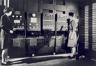
Predicting the movement of clouds, the intensity of storms, and the shifting of temperatures requires more than just looking at the sky. Numerical Weather Prediction (NWP) utilizes complex mathematical models of the atmosphere and oceans to forecast future weather conditions based on current observations. While the concept was first attempted in the 1920s, it was the arrival of computer simulation in the 1950s that finally allowed these models to produce realistic, actionable results.

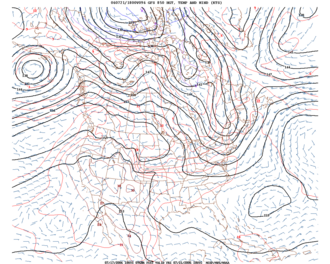
Today, global and regional forecast models are operated by various countries worldwide. These systems ingest massive amounts of data from radiosondes (weather balloons), satellites, and other observing systems to initialize their calculations. By applying the laws of physics to these datasets, scientists can generate everything from short-term daily forecasts to long-term climate projections used to understand global climate change.

A grid for a numerical weather model is shown. The grid divides the surface of the Earth along meridians and parallels, and simulates the thickness of the atmosphere by stacking grid cells away from the Earth's center. An inset shows the different physical processes analyzed in each grid cell, such as advection, precipitation, solar radiation, and terrestrial radiative cooling. — Weather models use systems of differential equations based on the laws of physics, which are in detail fluid motion, thermodynamics, radiative transfer, and chemistry, and use a coordinate system which divides the planet into a 3D grid. Winds, heat transfer, solar radiation, relative humidity, phase changes of water and surface hydrology are calculated within each grid cell, and the interactions with neighboring cells are used to calculate atmospheric properties in the future.

Key Facts

A prognostic chart of the North American continent provides geopotential heights, temperatures, and wind velocities at regular intervals. The values are taken at the altitude corresponding to the 850-millibar pressure surface. — A prognostic chart of the 96-hour forecast of 850 mbar geopotential height and temperature from the Global Forecast System

NWP relies on mathematical models based on physical principles like fluid motion and thermodynamics.
Modern forecasting requires some of the world's most powerful supercomputers to process vast datasets.
The current limit of reliable forecast skill for numerical models is approximately six days.
Ensemble forecasting is used to define uncertainty and extend the viable forecasting window.
Regional models have significantly improved tropical cyclone track and air quality predictions.

The Mechanics of Atmospheric Modeling

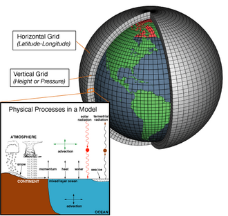
At its core, NWP works by dividing the planet into a 3D grid. Within each grid cell, the model calculates various atmospheric properties, including winds, heat transfer, solar radiation, relative humidity, and phase changes of water. These calculations are driven by systems of differential equations that represent the fundamental laws of physics.

The ENIAC main control panel at the Moore School of Electrical Engineering operated by Betty Jennings and Frances Bilas

Parameterization and Resolution

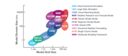
One of the greatest challenges in modeling is scale. Some atmospheric processes, such as the formation of individual cumulus clouds, occur at a scale too small to be explicitly included in a global grid. To account for these, scientists use parameterization—a method of representing these small-scale processes within the larger model framework.

Field of cumulus clouds, which are parameterized since they are too small to be explicitly included within numerical weather prediction

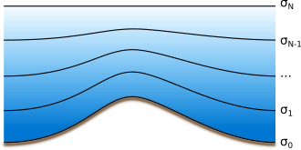
Models also vary in their spatial domains. While global models cover the entire planet, mesoscale models focus on smaller, specific regions. These mesoscale models often use specialized vertical representations, such as sigma coordinates, to better account for how the atmosphere interacts with complex terrain.

A sigma coordinate representation is shown. The lines of equal sigma values follow the terrain at the bottom, and gradually smoothen towards the top of the atmosphere. — A cross-section of the atmosphere over terrain with a sigma coordinate representation shown. Mesoscale models divide the atmosphere vertically using representations similar to the one shown here.

A plot of model domain size versus model grid size with several different types of numerical models arranged diagonally. — A comparison of different types of atmospheric models by spatial domain and model grid size

Improving Accuracy: MOS and Ensembles

Even the most advanced models can struggle to resolve fine details near the Earth's surface. To bridge this gap, meteorologists developed Model Output Statistics (MOS) in the 1970s and 1980s. MOS establishes a statistical relationship between the model's raw output and the actual conditions observed on the ground, helping to correct errors.

To address the inherent uncertainty in weather, ensemble forecasting became a standard practice in the 1990s. Instead of running a single simulation, meteorologists run multiple simulations with slightly different initial conditions. This "spread" of results helps define the level of uncertainty in a forecast, allowing for more reliable long-range predictions.

Two images are shown. The top image provides three potential tracks that could have been taken by Hurricane Rita. Contours over the coast of Texas correspond to the sea-level air pressure predicted as the storm passed. The bottom image shows an ensemble of track forecasts produced by different weather models for the same hurricane. — Top: Weather Research and Forecasting model (WRF) simulation of Hurricane Rita (2005) tracks. Bottom: The spread of NHC multi-model ensemble forecast.

Global Forecasting Systems and Applications

Different nations utilize various specialized models to provide localized and global coverage. For example, the North American Ensemble Forecast System integrates data from the US Global Forecast System, the Canadian Global Environmental Multiscale Model, and the European Integrated Forecast System, among others.

Comparison of Major Global and Regional Forecasting Systems
Organization/Region	Primary Model(s) Used	Key Characteristics
US National Weather Service	GFS, NAM, RAP, HRRR	Includes high-resolution hourly updates (RAP/HRRR)
Japan Meteorological Agency	MSM, LPS	Provides 3-hour and 1-hour updates with uncertainty estimation
European Centre (ECMWF)	IFS	Part of the North American Ensemble integration
China Meteorological Administration	CMA-MESO, Global Assimilation	Regional and global coverage
CPTEC (Brazil)	BRAMS, ETA	Specialized for South American regional modeling

Specialized Applications

Numerical models are not limited to general weather. They are critical for specific high-stakes scenarios:

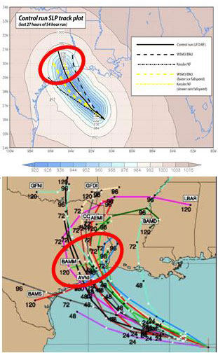
Tropical Cyclone Forecasting: Since 1978, dynamical models like the movable fine-mesh (MFM) model have been used to track hurricanes. While track forecasting has seen massive improvements, predicting the exact intensity of a cyclone remains a significant challenge.
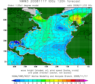
Ocean Surface Modeling: Models like Wavewatch III provide essential wind and wave forecasts for maritime safety.
Air Quality: Regional models help predict the movement of pollutants.
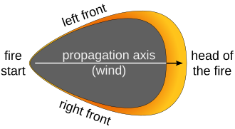
Wildfire Modeling: While atmospheric models struggle with the highly constricted areas of wildfire propagation, specialized models are used to track fire spread.

A WP-3D Orion weather reconnaissance aircraft in flight. — Weather reconnaissance aircraft, such as this WP-3D Orion, provide data that is then used in numerical weather forecasts.

A wind and wave forecast for the North Atlantic Ocean. Two areas of high waves are identified: One west of the southern tip of Greenland, and the other in the North Sea. Calm seas are forecast for the Gulf of Mexico. Wind barbs show the expected wind strengths and directions at regularly spaced intervals over the North Atlantic. — NOAA Wavewatch III 120-hour wind and wave forecast for the North Atlantic

Frequently Asked Questions

How do meteorologists collect data for these models?

Data is gathered from a variety of observing systems, including weather satellites, radiosondes (weather balloons), and other ground-based and airborne instruments like weather reconnaissance aircraft.

Why can't weather forecasts be accurate for more than a week?

Despite the massive power of modern supercomputers, the forecast skill of numerical weather models currently extends to only about six days due to the complexity of atmospheric variables and the limitations of initial data.

What is the difference between weather and climate modeling?

Both use similar physical principles, but weather models focus on short-term atmospheric conditions, while climate models are used for long-term projections to understand and project climate change.

What makes tropical cyclone intensity hard to predict?

While dynamical models have become excellent at predicting the track (path) of a hurricane, predicting its intensity remains difficult, with statistical methods often showing higher skill than dynamical guidance in this specific area.

What are the main factors that affect forecast accuracy?

Accuracy is primarily affected by the density and quality of the initial observations used as input, as well as inherent deficiencies or limitations within the numerical models themselves.